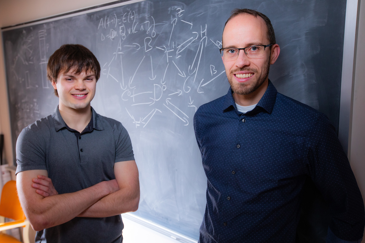
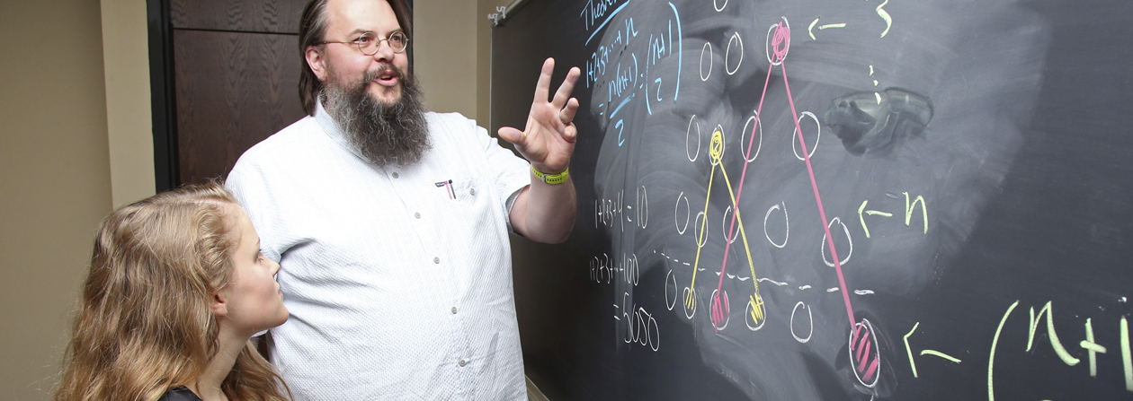
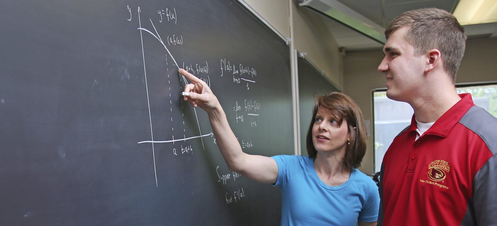
These chaos-fractal representations of the different sorts of genetic
material do in fact look different. They also have a lot of appearance
of similarity. This similarity comes from the fact that any
four-cornered chaos-game fractal will look somewhat like a subset of a
ramified cross.
All of the fractals above used the same number of iterations of the
chaos game, but they had to deal with differing amounts of input data.
For the shorter DNA strings the sequence data was reused until 2,000,000
points (or 20,000 shaded disks) were plotted. The gaps in the fractals
may be real but they may also be small sample size effects (if we are
thinking of them as part of a type of DNA). This suggests it would be
nice to get a model of the data and then plot a chaos fractal based on
the model. A simple Markov chain produced the fractal
,
and so we will look at deriving Markov
models from DNA and then plotting the chaos fractal of the Markov chain.
This serves to ``smooth'' the data.
We will use a simple Markov model, defined as follows. For a window
of size k, we will record all the patterns of k consecutive nucleotides
that occur, together with the distribution of the next nucleotide that
follows that pattern. The number k is the order of the Markov
model. Once we have fit a kth order Markov model to a given genetic
sample we will then use that Markov chain to generate a chaos fractal.
Starting with the pattern of k Cs, we generate a "next" nucleotide from
the Markov chain. We then move this new nucleotide into our
k-nucleotide window, bumping the oldest member of the window, and get a
new distribution of "next" nucleotides from the Markov chain. By
iterating this process we synthesizing DNA with the same (k+1)st order
statistics as the original sample. The result of using this fake DNA to
draw chaos fractals, for 2nd, 3rd, 4th, and 5th order Markov models, are
shown below.
Gene Source
|
Markov Chain Order
|
2
|
3
|
4
|
5
|
HIV
|
 |
 |
 |
 |
Maize
|
 |
 |
 |
 |
Chloro- plast
|
 |
 |
 |
 |
Drosophila
|
 |
 |
 |
 |
Tobacco mosaic virus
|
 |
 |
 |
 |
Mouse MHC
|
 |
 |
 |
 |
In this section we begin by simply repeating
the process of extracting a Markov model from DNA and using it to drive
a chaos game for six whole microbial genomes. To show more detail these
are 240x240 gif files: widen your browser.
Gene Source (Whole Genome)
|
Markov Chain Order
|
3
|
4
|
5
|
Archaeoglobus fulgidus
|
 |
 |
 |
Borrelia burgdorferi
|
 |
 |
 |
Haemophilus influenzae
|
 |
 |
 |
Heliobacter pylori
|
 |
 |
 |
Methanococcus jannaschii
|
 |
 |
 |
Mycobacterium tuberculosis
|
 |
 |
 |
In this section, we compute the fifth order Markov models of the DNA
for all six of our whole microbial genomes, create chaos fractals with
hit counts, and then let the differential hit count dictate the color of
a difference fractal. The color that is ahead at any given pixel is
dictated by the red and green row/column labels, as follows:
Archaeoglobus fulgidus | AF |
Borrelia burgdorferi | BB |
Haemophilus influenzae | HI |
Heliobacter pylori | HP |
Methanococcus jannaschii | MJ |
Mycobacterium tuberculosis | MT |
The difference fractals are indexed with half size version of the
fifth-order Markov chaos game. The difference for two microbial genomes
is given by the intersection of the row and column where their fifth
order Markov fractals intersect.
Fifth order Markov chaos fractal differences |
|
|
AF |
BB |
HI |
HP |
MJ |
|
|
 |
 |
 |
 |
 |
BB |
 |
 |
HI |
 |
 |
 |
HP |
 |
 |
 |
 |
MJ |
 |
 |
 |
 |
 |
MT |
 |
 |
 |
 |
 |
 |
At this point we drop the four cornered chaos game and look at other
sorts of fractal-generating processes. The fractals at the end of this
section are a restricted type of contraction map fractal (as is the
chaos game). There are three issues here: the generation method for the
fractals, the way we drive the fractals with our DNA data, and finally
the way we located the fractals so that they had the property of
separating DNA with stop codons from DNA without stop codons.
Disclaimer: the DNA used for these fractals was maximally random
simulated DNA - which is probably the most difficult case, of which we
will say more later.
The Fractals
A contraction map is a map f(x), in this case from the plane
to itself, that has the property that for any two points x,y, the
distance from x to y is at least the distance from f(x) to f(y). In
other words, all distances are contracted by this map. It is a theorem
that such a map has a unique fixed point p so that f(p)=p and the map
contracts the whole plane toward that point.
Michael Barnsley showed that you can use contraction maps to generate
fractals in the following way. Much as with the chaos game, you plot
moving points. Instead of moving toward the corners of a square or a
triangle selected at random, you instead select contraction maps at
random from a list of contraction maps. The unique fixed point replaces
the corners of the polygon. The 20 fractals at the end of this section
were generated in this fashion.
For our DNA driven fractals we need a large source of random
contraction maps. This is because we will search for fractals that can
separate different types of DNA and so need a space of fractals which in
turn requires a space of contraction maps. We chose to use
similitudes. Similitudes, in the plane, are a four-parameter
family of contraction maps. The first parameter is an angle t through
which the plane is rotated. The second and third parameters are the
coordinates of a vector through which the plane is displaced. The
fourth parameter is a shrink factor in the range from 0 to 1 which is
used to contract the plane toward the origin. Since rotation and
translation are distance preserving, it follows that a rotation, a
displacement, and then a contraction form a contraction map. The
mathematical form of a similitude is:
The fractals we are using have eight similitudes. We measure the
average position of the moving point and the maximum distance the point
gets from that average position to get a "center" and "radius" that can
be used to normalize the resulting fractal.
Driving the fractals with DNA
The "DNA" used to drive these fractals comes from two random sources.
One is a maximum entropy source with 25% each of CGAT. The other is a
maximum entropy source that avoids the triples TAA, TGA, and TAG,
i.e. stop codons. This latter source is implemented by generating, with
equal probability, any letter that does not create a stop codon in the
reading frame starting with the first character generated.
We read the DNA in triples mapping the 64 possible triples onto one
of right possible similitudes with a lookup table. For the first of the
20 fractals below the lookup table was:
CCCCCCCCCCCCCCCCGGGGGGGGGGGGGGGGAAAAAAAAAAAAAAAATTTTTTTTTTTTTTTT
CCCCGGGGTTTTAAAACCCCCGGGGTTTTAAAACCCCGGGGTTTTAAAACCCGGGGTTTTAAAA
CGATCGATCGATCGATCGATCGATCGATCGATCGATCGATCGATCGATCGATCGATCGATCGAT
1333714743627132617277121322763137276232223623277726627337713321
So, for example, the triple GCC caused the
fractal to use similitude 6. This scheme
lest us drive the eight similitudes with 64 DNA based features. At this
point it is probably worth noting that this selection of features, in
this case DNA triples, is a major area for exploration. Using different
features to drive the similitudes opens up many possible fractal
tools.
Searching for separating fractals.
The data structure we used to store fractals is a list of eight
similitudes and a 64 element lookup table mapping DNA triples onto those
similitudes. This means each fractal has 8x4=32 real parameters and 64
three-bit integer parameters. This is a very large search space.
Because of this we used a genetic algorithm to search the space of
possible fractals.
Genetic algorithms operate by starting with a collection of random
objects (in this case fractals). Our genetic algorithm would these
select four fractals and sort them from best to worst in a manner
described below. The two best fractals were then copied over the two
worst. Within those copies a random suffix of the list of eight
similitudes and a random middle segment of the lookup table were
exchanged, a process called crossover. One of the two new
fractals then has a small amount added or subtracted to one of its
similitude parameters, selected at random, while the other had one entry
of its lookup table changed, two different sorts of mutation.
Repeated many times, this process locates high quality fractals.
So, what quality measure are we using? In this case we sent in the
stop codon free and stop codon containing DNA in blocks of from 50-400
triples. The mean position of points plotted for each sort of random
source were computed and the measure of quality was taken to be the
Euclidean distance between these means. Red points result from
stop-codon free DNA, green points from stop-codon containing DNA. While
the means are separate, the red and green domains mix: they don't overlap
much though - overlap would be yellow in our coding scheme. We give the
best-of-run fractals from 20 different runs of the genetic algorithm.
Enjoy the fractals.
In this section we take the whole genome of mycobacterium
tuberculosis and use it, both in frame and out of frame, to replace the
two random sources in the previous section. Below, we show the output
of three runs of the genetic algorithm in three forms. The leftmost gif
shows the raw separation, red for in frame and green for out-of-frame.
The middle gif displays this same image run through a smoothing filter
to widen the yellow boundary areas where the fractal system is not in
the attractor of either reading frame. The third image is the fractal
with each of the eight similitudes color coded with on of the eight
possible RGB colors. All of the below are thumbnails, click on them to
obtain full-sized pictures.
In this section we take the whole genome of mycobacterium
tuberculosis and a good chunk of human chromosome 22 and compute the
difference between the 5th order Markov model of the DNA and the DNA.
To do this two chaos games are run and hit counts for pixels compiled.
These chaos games are then used as strengths of a red and a green
channel. The red channel is the Markov chain chaos game, the green
channel one driven directly by data. Red and green blend to make
yellow. Finally areas hit by neither chaos game are set to a constant
blue value. To prevent outliers from dominating, the data are truncated
to twice the sample variance of the hit count in each channel before
they are superimposed.
 |
 |
Tuberculosi |
H. Sapiens |
Here we give a pair of images (click for double size) that use a
histogrammatic count of the 6-mers (length six DNA substrings) of the
Mycobacterium tuberculosis genome in the correct reading frame and in an
incorrect reading frame to drive a six similitude Barnsley type
contraction may fractal. The fractal pictures look different with the
yellow lobe being larger for the out-of-frame data while the cyan lobe
is larger got the in-frame data.
 |
 |
In frame. |
Out of frame. |